

Introduction
FASTA format is a widely used text-based format for representing nucleotide sequences. Understanding the composition of these sequences is crucial in various fields of biological research, particularly in genomics and bioinformatics. One of the key metrics derived from nucleotide sequences is the GC content, which is the percentage of nucleotide bases in a DNA molecule that are either guanine (G) or cytosine (C).
Importance of GC Content
GC content is an important parameter that can affect the stability and structure of DNA, influence gene expression, and provide insights into the evolutionary relationships between organisms. High GC content can lead to increased stability of DNA due to stronger hydrogen bonding between G and C bases compared to A and T bases. Conversely, low GC content may be associated with certain genomic characteristics, such as increased mutation rates or specific adaptations to environmental conditions.
Overview of Bio.SeqIO Module
The Biopython library offers a comprehensive suite of tools for biological computation. The Sequence Input/Output, Bio.SeqIO module is particularly useful for reading and writing sequence data in various formats, e.g., FASTA, GenBank. This module provides a convenient interface for accessing sequence records and their associated annotations based on Biopython Tutorial and Cookbook, provide objects to represent biological sequences.
Usage of Bio.SeqIO
The Bio.SeqIO module allows for straightforward manipulation of sequence data. Users can read FASTA files, extract sequences, and perform operations on them with minimal code. The following functions are central to using Bio.SeqIO:
- SeqIO.parse(): This function reads sequence records from a file in a specified format, allowing iteration over each record. Each sequence record has metadata, such as an ID and description, and includes the sequence data itself.
- SeqIO.write(): This function writes sequence records to a specified output file in a designated format.
from Bio import  SeqIO

file_path = "example.fasta"
records = SeqIO.parse(file_path, "fasta")
for record in records:
    print("Header:", record.id)
    print("Sequence:", record.seq)
    print()

#Output
Header: sp|P25730|FMS1_ECOLI
Sequence: MKLKKTIGAMALATLFATMGASAVEKTISVTASVDPTVDLLQSDGSALPN

Header: sp|P15488|FMS3_ECOLI
Sequence: LTLSNTGVSNTLVGVLTLSNTSIDTVSIASTNVSDTSKNGTVTFAHETNNS
Biopython Program to Calculate GC Content of a FASTA File
Requirements
- A text editor or integrated development environment (IDE) for writing and executing Python scripts (e.g., VSCode, PyCharm, Jupyter Notebook).
- This protocol can be executed on any operating system that supports Python, including Windows, macOS, and Linux
- Dependencies: Ensure that Biopython is installed in your Python (version 3.6 or higher) environment. If not installed, you can do so by running the following command in your terminal via pip (pip install biopython) or download it from python.org.
Here’s the FASTA (sequences.fasta) file that will be used in this tutorial.
>ref|NC_005213.1|:883-2691
ATGAAAAAGCCCCAACCCTATAAAGATGAAGAGATATATTCTATTTTAGAAGAGCCCGTAAAACAATGGT
TTAAAGAGAAATACAAAACATTCACTCCCCCACAAAGGTATGCAATAATGGAAATACATAAAAGGAACAA
TGTTTTAATTTCTTCCCCCACAGGTTCGGGAAAAACGTTAGCAGCGTTTTTAGCTATAATAAATGAATTA
ATAAAGTTATCTCATAAAGGAAAATTAGAAAATAGAGTTTATGCCATTTATGTTTCTCCATTAAGAAGTT
TAAATAACGATGTAAAGAAAAACTTAGAAACTCCATTAAAAGAAATAAAAGAAAAAGCGAAAGAGCTTAA

>ref|NC_005214.1|:1000-1900
ATGCGTACGTTGACCTTGAATGGCTTAGCTCAGTGACGTAGCTGTAACGGTACGCGTGTATACATCC
TTAATCCGTTAGCAGCTCTGACGATGCCGATCCTGTAAGTTGACGTAAGTCGTGATGACGCGTCTAC
TACGATACATGCTGTGAGGCCATCAGTCTGACATCGATCGTACGCGTACGTACGTAAGGAGCTAACG
TAACTGACGTATACGTGACGAGTTGACGATCGAACGATCGAATCGTCGATGATCGACGACGTACGAC
TAGGTAACGTAGCTAGCGTGACGCGTGATGACGAGCAGACGAGCGTGATCGTACGATCAGCTTACGT

>ref|NC_005215.1|:1500-2800
ATGACGTAGCGTACGTAGCTGATCGTAGCGTGATGCTACGCGTACGTAGCGTAGCTGATCGTAGCAG
TTAGCTAGCTAGCTAGTAGCTAGTCAGTGATCGTACGTAGCGTACGATGACTAGCTAGCGTGATGAC
GTTAGCTAGCTAGTAGCTAGCGTAGCTAGTACGTAGCGTACGTTAGCTGACTAGCTGAGCTAGTAGG
CAGATCGTACGGTACGTAGCGTACGGTACGTACGTAGCTAGCTGATGATGCGTAGCTGACTGAGCTT
GAGCTGACTACGTGACGTAGCAGCGTGAGTACGATCGTACGACGATCGTACGTACGATCGTGACGT

>ref|NC_005216.1|:2000-3900
ATGTACGTAGCTAGTACGTTAGGTCAGCTGACGGTACGGTACGTAGGAGCTAGTCGTCGAGCGTTAG
TAGCTAGCGTAGTGACGACGTACGAGTACGTGACGTAGTAGCTGACGTCGATGACGATCGTCGACGT
ACGTTAGCTAGGTCAGTACGTAGCGTACGTAGTGAGCGTCGACGATCGACGTTAGCAGTGACGAGTC
GACGACGTACGAGTAGCGTACGTTAGCTAGCTGATGACGTCGACGATCGTACGAGTGAGTCGAGTAC
GTAGACGTACGTCGTCGATCGTAGCTAGCTGACGTACGTCGTGATGTCGTAGCTAGCGACGTCGAT

>ref|NC_005217.1|:1200-2500
ATGTCGATAGTGACGTGTCGACTGACGTAGCGTACGTTAGTCGACGTAGTACGATGATGACGTAGC
TAGTGAGTAGTAGGTCGACGTTGACGATAGTCAGCGTACGATCGACGTCGACGTAGTAGCTGACGTA
TAGTAGGTCGTAGTGATGTCGAGCTAGCTGACGTAGTGACGACGAGTCGTCGACGTTAGCGTAGCTG
CTGACGTGACGATGAGCTAGTAGTCGACGTAGCGTGACGAGCTAGTGACGTTAGTCGACGTGATCGT
GTAGCTAGCTAGTGTCGAGTCGTAGCTAGCTGACGACGGTAGTACGTGACGTAGTACGACGTAGCT
Counting GC Content
The calculation involves the use of Bio.SeqUtils.GC() function for the GC percentage calculation rather than: gc_content = (sequence.count(“G”) + sequence.count(“C”)) / len(sequence) * 100.
# Import the necessary modules
from Bio import SeqIO
from Bio.SeqUtils import GC

# Define the path to the FASTA file
fasta_file_path = "sequences.fasta"
gc_content_dict = {}

# Parse the FASTA file
for record in SeqIO.parse(fasta_file_path, "fasta"):
    sequence = str(record.seq)  # Convert sequence to a string
    gc_content = GC(sequence)  # Calculate GC content using Bio.SeqUtils.GC()
    gc_content_dict[record.id] = gc_content

# Print GC content for each sequence
for seq_id, gc in gc_content_dict.items():
    print(f"Sequence ID: {seq_id}, GC Content: {gc:.2f}%")
Output
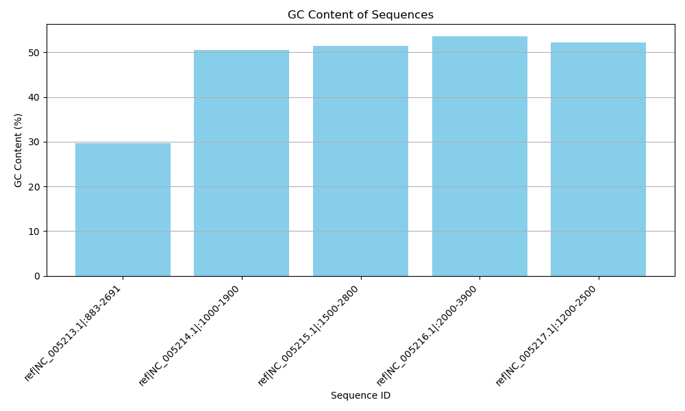
Sequence ID: ref|NC_005213.1|:883-2691, GC Content: 29.71%
Sequence ID: ref|NC_005214.1|:1000-1900, GC Content: 50.45%
Sequence ID: ref|NC_005215.1|:1500-2800, GC Content: 51.50%
Sequence ID: ref|NC_005216.1|:2000-3900, GC Content: 53.59%
Sequence ID: ref|NC_005217.1|:1200-2500, GC Content: 52.25%
GC content graph
To plot the GC content graph, will be using matplotlib (pylab) module.
from Bio import SeqIO
from Bio.SeqUtils import GC
import matplotlib.pylab as plt #matplotlib (pylab) to plot the graph

fasta_file_path = "sequences.fasta"
gc_content_dict = {}

for record in SeqIO.parse(fasta_file_path, "fasta"):
    sequence = str(record.seq)
    gc_content = GC(sequence)
    gc_content_dict[record.id] = gc_content

for seq_id, gc in gc_content_dict.items():
    print(f"Sequence ID: {seq_id}, GC Content: {gc:.2f}%")

# Plotting the GC content
plt.figure(figsize=(10, 6))  # Set the figure size
plt.bar(gc_content_dict.keys(), gc_content_dict.values(), color='skyblue')  # Create a bar plot
plt.title('GC Content of Sequences')  # Set the title
plt.xlabel('Sequence ID')  # Set the x-axis label
plt.ylabel('GC Content (%)')  # Set the y-axis label
plt.xticks(rotation=45, ha='right')  # Rotate x-axis labels for better visibility
plt.tight_layout()  # Adjust layout to make room for labels
plt.grid(axis='y')  # Add a grid for better readability

# Show the plot
plt.show()
Summary
The article provides a detailed guide on calculating GC content in FASTA files using the Biopython library. It highlights the significance of GC content in molecular biology, affecting DNA stability and gene expression. The tutorial outlines the use of the Bio.SeqIO module for reading FASTA files and demonstrates how to compute GC content using the Bio.SeqUtils.GC() function. Additionally, it includes code examples for visualizing the GC content through bar plots using the Matplotlib library.
Reference
- Cock, P. J. A., et al. Biopython Tutorial and Cookbook. Biopython.org, 2009.
